Searching code on Mac

Most of the heavy lifting for data processing and GIS is done on linux computers, but a lot of development and nearly all of my writing and thinking happens on a Mac laptop. There are a lot of tools that I rely heavily on for organizing ideas and information.

I also rely heavily on search for finding things, using basic Spotlight and the excellent HoudahSpot. These tools are great for searching file names of any sort, but Spotlight wwill only search and show previews for files with extensions it recognizes, regardless of what the file type actually is. I use *.Rmd for R markdown files and *.rbat for certain kinds of R scripts, and has been frustrating to be unable to search them.

After reading a bunch of articles and some trial and error, I’ve figured out how to teach Spotlight to recognize text files with custom extensions. Most of the search results I found gave information that does not work with newer versions of Mac OS because of changes to the security settings. The following works on Catalina.

First figure out what your file types are being classified as. You’ll need a terminal for this and subsequent steps.

mdimport -d1 -t filename

will tell you what Spotlight thinks your file is. I tried three different file types, all of which are plain text.

  • Imported ‘myfile.R’ of type ‘com.apple.rez-source’ with plugIn /System/Library/Spotlight/RichText.mdimporter.
  • Imported ‘myfile.Rmd’ of type ‘dyn.ah62d4rv4ge81e5pe’ with no plugIn.
  • Imported ‘myfile.rbat’ of type ‘dyn.ah62d4rv4ge81e2xbsu’ with no plugIn.

The *.R file was recognized as text, and Spotlight knew to use the RichText.mdimporter to process it, but the other two file types were recognized as “dyn.randomstring” and Spotlight couldn’t figure out what to do with them.

It’s straightforward to modify RichText.mdimporter to create your own custom Spotlight importer. I renamed mine to RCode.mdimporter but you may not need to rename it since you are putting the new importer in your personal library, and not touching the system file.

First, make a directory to hold Spotlight files in your local library, and then copy the system Spotlight importer to it.

mkdir ~/Library/Spotlight
cp -r /System/Library/Spotlight/RichText.mdimporter ~/Library/Spotlight/RCode.mdimporter

Now open the file ~/Library/Spotlight/RCode.mdimporter/Contents/Info.plist with your favorite text editor. Refer back to the results of the first command, because you’ll need the “dyn.randomstring” information. Look for the section on LSItemContentTypes and add the content type for your text files to it, in the same format as the other types listed. For my *.Rmd and *.rbat files, the lines to add are:

<string>dyn.ah62d4rv4ge81e5pe</string>
<string>dyn.ah62d4rv4ge81e2xbsu</string>

but use your own results from mdimport.

Save and close that file. The only thing left is to tell Spotlight to reindex your files using the modified definitions.

mdimport -r ~/Library/Spotlight/RCode.mdimporter

It took a few minutes to complete, but now when I search, I get full-text preview in HoudahSpot for my R code files.
Files and memory

I’m still working with that 6TB of data, and likely will be for a long time. The data are divided up by time: full spatial extent for a few time periods. The research group would also like to have time series for a particular location, but I can’t load all the data into memory. My current approach is to load a dataset, then save it as smaller chunks (expect more on file formats and save/load options later). The chunks are small enough in spatial extent that I can open them all and assemble a time series.

Looping over a large number of files in R, doing things with them, then writing them out again can lead to slow memory leaks, even if files are over-written. Hadley Wickham talks about memory management in R in Advanced R. I spent some time poking around with the pryr package, just out of curiousity, but there’s an easier solution: stick all the heavy lifting into a function. As long as the function doesn’t return something that includes its environment, the memory is freed upon exit.

All the file handling (reading and writing) goes into the function.


loadfn <- function(filepatt, outname) {

  # list all the files matching the specified pattern

  filelist <- list.files(pattern=filepatt)

  fulldata <- vector(length(filelist), mode="list")

  for(thisfileno in seq_along(filelist)) {

    load(filelist[thisfileno]) # loads as thissave

    fulldata[[thisfileno]] <- thissave

  }


  fulldata <- do.call("cbind", fulldata)


  # do some other processing

  # rename the object and save it

  assign(outname, fulldata)

  save(list=c(outname), file=paste0(outname, ".RDA"))

  invisible()

}

Then the function is called for the full list of possible patterns.


for(thispatt in filepatterns) {

  loadfn(thispatt, paste(thispatt, "series", sep=".")

}

No clean-up, no memory leaks. The operating system no longer kills my process every time I leave it.

File compression

I have about 6TB of climate data to manage, and more on the way. Besides a decent array of hard drives and a clever backup strategy, what tools can I use to help maintain these data in a useful way? They’re in NetCDF files, which is a decent (if non-user-friendly) way to maintain multidimensional data (latitude, longitude, time).

We’re mostly interested in summaries of these data right now (CLIMDEX, BIOCLIM, and custom statistics), and once these are calculated the raw data themselves will not be accessed frequently. But infrequently is not the same as never, so I can’t just put them on a spare hard drive in a drawer.

What are the compression options available to me, and what is the trade-off between speed and size for the NetCDF files I’m working with?

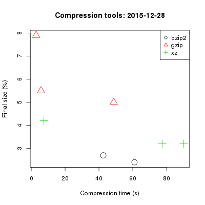
There are three major file compression tools on linux, the venerable gzip, bzip2, and the newer xz. I tried them out on a 285MB NetCDF file, one of the very many I’m working with. I included most compression (-9) and fastest (-1) options for each of the three tools, plus the default (-6) for gzip and xz. bzip2 doesn’t have the same range of options, just best (the default) and fast.

There wasn’t a huge difference in compression for this type of file, with the best (bzip2 -best) resulting in 2.4% of the original, and the worst (gzip -1) in 7.9% of the original size.

Speed, though: anywhere from 2.9 to 90.0 seconds to compress a single file. Uncompression time was about 1.6 seconds for gzip and xz regardless of option, and 3.2-3.6 for bzip2.

Compression tool results

For this file format, xz was useless: slow and not the most effective. bzip2 produced the smallest files, but not by a huge amount. gzip was fastest, but produced the largest files even on the best mode.

This matches what I expected, but the specifics are useful:

  • Using bzip2 -best I could get one set of files from 167GB to 4GB, but it would take 9.5 hours to do so.
  • Using gzip -1 I could get that set of files down to 13GB, and it would only take 24 minutes.

I think that’s a fair trade-off. The extra 9 hours is more important to me than the extra 9GB, and accessing a single file in 1.5 seconds instead of 3.5 also improves usability on the occasions when we need to access the raw data.