Searching code on Mac

Most of the heavy lifting for data processing and GIS is done on linux computers, but a lot of development and nearly all of my writing and thinking happens on a Mac laptop. There are a lot of tools that I rely heavily on for organizing ideas and information.

I also rely heavily on search for finding things, using basic Spotlight and the excellent HoudahSpot. These tools are great for searching file names of any sort, but Spotlight wwill only search and show previews for files with extensions it recognizes, regardless of what the file type actually is. I use *.Rmd for R markdown files and *.rbat for certain kinds of R scripts, and has been frustrating to be unable to search them.

After reading a bunch of articles and some trial and error, I’ve figured out how to teach Spotlight to recognize text files with custom extensions. Most of the search results I found gave information that does not work with newer versions of Mac OS because of changes to the security settings. The following works on Catalina.

First figure out what your file types are being classified as. You’ll need a terminal for this and subsequent steps.

mdimport -d1 -t filename

will tell you what Spotlight thinks your file is. I tried three different file types, all of which are plain text.

  • Imported ‘myfile.R’ of type ‘com.apple.rez-source’ with plugIn /System/Library/Spotlight/RichText.mdimporter.
  • Imported ‘myfile.Rmd’ of type ‘dyn.ah62d4rv4ge81e5pe’ with no plugIn.
  • Imported ‘myfile.rbat’ of type ‘dyn.ah62d4rv4ge81e2xbsu’ with no plugIn.

The *.R file was recognized as text, and Spotlight knew to use the RichText.mdimporter to process it, but the other two file types were recognized as “dyn.randomstring” and Spotlight couldn’t figure out what to do with them.

It’s straightforward to modify RichText.mdimporter to create your own custom Spotlight importer. I renamed mine to RCode.mdimporter but you may not need to rename it since you are putting the new importer in your personal library, and not touching the system file.

First, make a directory to hold Spotlight files in your local library, and then copy the system Spotlight importer to it.

mkdir ~/Library/Spotlight
cp -r /System/Library/Spotlight/RichText.mdimporter ~/Library/Spotlight/RCode.mdimporter

Now open the file ~/Library/Spotlight/RCode.mdimporter/Contents/Info.plist with your favorite text editor. Refer back to the results of the first command, because you’ll need the “dyn.randomstring” information. Look for the section on LSItemContentTypes and add the content type for your text files to it, in the same format as the other types listed. For my *.Rmd and *.rbat files, the lines to add are:

<string>dyn.ah62d4rv4ge81e5pe</string>
<string>dyn.ah62d4rv4ge81e2xbsu</string>

but use your own results from mdimport.

Save and close that file. The only thing left is to tell Spotlight to reindex your files using the modified definitions.

mdimport -r ~/Library/Spotlight/RCode.mdimporter

It took a few minutes to complete, but now when I search, I get full-text preview in HoudahSpot for my R code files.

Unclassy behavior

You’re never too experienced to get caught out by one of R’s quirks. Today: dates! Creating a sequence of dates is easy. Looping over a sequence of dates is also easy, right?

datelist <- seq(as.Date("2020-01-01"), as.Date("2020-01-05"), by="day")

for(thisdate in datelist) {
    print(thisdate)
}

But, no.

[1] 18262
[1] 18263
[1] 18264
[1] 18265
[1] 18266

That is not so helpful, especially if you are actually trying to do something with those dates.

It turns out that R loses the class information on loop indices, so the Date class gets converted back to integer (days since 1970-01-01).

Two potential solutions: convert the integer back into a date, or loop over the index rather than the vector of dates directly.]

# option 1

for(thisdate in datelist) {
print(as.Date(thisdate, origin = "1970-01-01"))
}

[1] "2020-01-01"
[1] "2020-01-02"
[1] "2020-01-03"
[1] "2020-01-04"
[1] "2020-01-05"

# option 2

for(i in seq_along(datelist)) {
thisdate <- datelist[i]
print(thisdate)
}
[1] "2020-01-01"
[1] "2020-01-02"
[1] "2020-01-03"
[1] "2020-01-04"
[1] "2020-01-05"

Both solutions work; neither is quite as elegant as a direct loop.

While I got caught out by dates in a for-loop, this can occur with other classed objects.

Incidentally, I also stumbled on another unexpected occurrence.

thisdate <- datelist[1]

print(thisdate)
[1] "2020-01-01"
cat(thisdate, "\n")
18262

If you use cat() as a way to avoid the line numbers, or within code to print to screen, you may also lose the class information.

Posted in |

Clean and new

R 4.0.0 was just released! Binaries have magically appeared in the usual places.

But when you install a major upgrade like 3.6 to 4.0, you find yourself with a fresh, clean, empty, package library. Yikes!

Fortunately, installing all your old CRAN packages is easy, because your old library hasn’t been deleted and you can reference it.

Mac OSX saves the complete library with version number, so you need to get not just the path to your library, but the correct path to the previous version, because the 4.0 path will have only base packages.

# use .libPaths() to get the base directory, for me on OSX
#"/Library/Frameworks/R.framework/Versions/4.0/Resources/library"
# and replace 4.0 with appropriate prior version
pkglist <- list.files("/Library/Frameworks/R.framework/Versions/3.6/Resources/library/")

# it would be more sensible to remove base packages FIRST
basepkg <- c('base', 'compiler', 'datasets', 'graphics', 'grDevices', 'grid', 'methods', 'parallel', 'splines', 'stats', 'stats4', 'tcltk', 'tools', 'utils')
pkglist <- pkglist[!(pkglist %in% basepkg)]
install.packages(pkglist)

Rich Shepard prompted me to look into the situation on linux, because it is different. There, the library directory doesn’t change, so you simply need to list its contents. On my server, .libPaths() returns two results, so here’s one way to get the package list from multiple locations.

# get list of packages from the library
pkglist <- unlist(lapply(.libPaths(), list.files))

# it would be more sensible to remove base packages FIRST
basepkg <- c('base', 'compiler', 'datasets', 'graphics', 'grDevices', 'grid', 'methods', 'parallel', 'splines', 'stats', 'stats4', 'tcltk', 'tools', 'utils')
pkglist <- pkglist[!(pkglist %in% basepkg)]
install.packages(pkglist)

I don’t know how this works on Windows, but I would be happy to add that information if someone shares their experience.

Then go get coffee, because it will take a while.

This doesn’t address GitHub or other packages, and that’s where it gets complicated. I for one don’t remember where I got all that other stuff!

What to do? Well, on my system install.packages() returned three warnings:

  1. Packages that couldn’t be installed.
  2. Base packages that shouldn’t be separately installed (also included in 1.) [EDIT: I moved the check for base packages to the original pkglist specification above, because there’s no reason to even try to install these.]
  3. Packages that are on CRAN but threw errors. This is often because some system component needs to be updated as well, and requires human intervention.

The warnings provide neat comma-separated lists of package names (except they use curly quotes WHY EVEN), so it’s fairly easy to create a list of everything in 1 that’s not part of 2.

notinstalled <- c( [list from warning message] )

basepkg <- c('base', 'compiler', 'datasets', 'graphics', 'grDevices', 'grid', 'methods', 'parallel', 'splines', 'stats', 'stats4', 'tcltk', 'tools', 'utils')

notinstalled <- notinstalled[!(notinstalled %in% basepkg)]

Here’s where it gets messy. Some of those packages are on GitHub, but you need to know the repository to install them using devtools. I don’t know that! Some of them are on CRAN but obsolete and can’t be installed. And some of them came from who-knows-where.

We can at least try to automatically install them from GitHub using the githubinstall package from CRAN, which will try to look up the repository name as well. It will list all the repositories with packages of that name, and if it can’t find an exact match will list similar matches. Multiple repo options require human intervention, but if there’s only one we can try to install it.

First see which packages have exactly one match on GitHub. Try to install those, and make a list of which ones failed.

# install.packages("githubinstall")
library("githubinstall")
notinstalled.gh <- lapply(notinstalled, gh_suggest)
notinstalled <- notinstalled[sapply(notinstalled.gh, length) > 1]

notinstalled.gh <- notinstalled.gh[sapply(notinstalled.gh, length) == 1]
gh.out <- lapply(notinstalled.gh, function(x)try(githubinstall(x, dependencies = TRUE, ask = FALSE)))
gh.failed <- notinstalled.gh[sapply(gh.out, function(x)inherits(x, "try-error"))]

And now, you have almost everything freshly installed on your R 4.0 system. There are three things left for you to deal with:

  1. The packages that install.packages() threw error messages for.
  2. The packages in notinstalled that weren’t cleanly matched on GitHub, and might have come from who-knows-where.
  3. The packages in gh.failed – on my system, there were three, and they all had dependencies that couldn’t be installed for whatever reason.

If all you use is CRAN packages, the first step might be all you need. If you’re like me and accumulate packages from all over, you might have a bit more work to do. Or you might decide you don’t care, and will ignore those lost sheep until you need them…

This started as a twitter thread, and rmflight suggested a couple of tools that may automate the process: reup and yamlpack. I haven’t tried either; I wanted to see all the intermediate steps myself. The packages that need human intervention are going to need that regardless, but that might make them easier.

For what it’s worth, of the 1136 packages installed on my laptop, one is on CRAN but threw an error, three were found on GitHub but couldn’t be installed, and seventeen more need to be tracked down. (Edit: most of those seventeen have been removed from CRAN because they aren’t being maintained; the rest I don’t actually care about.)
Posted in | Tagged |

Permutation tests

I answered a question about spatial pattern testing on the R-sig-geo email list. Designing your own permutation test is (can be?) fun and easy, and I thought I’d save it here for future reference.

Why permutation tests? You can get at exactly what you want to know, which can be especially useful with complex spatial questions.

The question: which are closer on average to points in A, points in B or points in C?

Null hypothesis: mean distance from B to A is equal to mean distance from C to A.

I’ve adapted the example slightly from the original question on the mailing list.

library(spatstat)

set.seed(2019)

A <- rpoispp(100) ## Base set
B <- rpoispp(50) ## First set of points
C <- rpoispp(50) ## Second set of points

ABd <- crossdist(A, B)
ACd <- crossdist(A, C)

mean(ABd)
# 0.5168865
mean(ACd)
# 0.5070118

Are the two distances different?

One way to approach this with a permutation test is to keep the points in B and C where they are, but shuffle the assignment to B or C. That formulation might be appropriate if you're working with trees, where the trees are where they are but you're concerned with whether species B is closer to species A than another species is. (There are multiple ways to approach this question, but I like permutation tests.)

The basic procedure, then, is to reorder the point labels a bunch of times, and take the mean resampled distances. Then compare the true difference in distances to the permuted difference in distances to see where the true distance falls in the overall distribution.

The thing about using this method is that it assumes that the trees don't move, and so takes into account the intrinsic structure of the tree spatial pattern.

nperm <- 999
permout <- data.frame(ABd = rep(NA, nperm), ACd = rep(NA, nperm))

# create framework for a random assignment of B and C to the existing points

BC <- superimpose(B, C)
B.len <- npoints(B)
C.len <- npoints(C)
B.sampvect <- c(rep(TRUE, B.len), rep(FALSE, C.len))

set.seed(2019)
for(i in seq_len(nperm)) {
B.sampvect <- sample(B.sampvect)
B.perm <- BC[B.sampvect]
C.perm <- BC[!B.sampvect]

permout[i, ] <- c(mean(crossdist(A, B.perm)), mean(crossdist(A, C.perm)))
}

boxplot(permout$ABd - permout$ACd)
points(1, mean(ABd) - mean(ACd), col="red")

table(abs(mean(ABd) - mean(ACd)) >= abs(permout$ABd - permout$ACd))
# FALSE TRUE
# 573 426

sum(abs(mean(ABd) - mean(ACd)) >= abs(permout$ABd - permout$ACd)) / nperm
# 0.4264264

The difference between ACd and ABd is indistinguishable from that obtained by a random resampling of B and C.

Or, there is no apparent difference in the mean distance of B to A or C to A.

Which is reassuring, since A, B, and C were all randomly generated.

Stuck on rgdal

Update: Thanks to Colin Rundel figuring out the problem and Roger Bivand implementing it, the devel version of rgdal (revision 758) on R-Forge installs beautifully.


I updated all of my linux computers to Fedora 28, and now can’t install rgdal.

I can install sf with no problems, so it isn’t an issue with GDAL or with proj.

I checked with Roger Bivand, the package maintainer, who asked me to confirm whether I could install sf, to make sure it wasn’t a dependency issue, and to post the logs online, then ask on the R-sig-geo mailing list. I’m putting the full problem here, and the abbreviated version on the mailing list.

I’d appreciate any thoughts: I rely very heavily on the incredibly useful rgdal package.


Fedora packages installed (fc28):

gdal 2.2.4-2
proj 4.9.6-3
gcc 8.1.1-1


R information:


> sessionInfo()
R version 3.5.0 (2018-04-23)
Platform: x86_64-redhat-linux-gnu (64-bit)
Running under: Fedora 28 (Workstation Edition)

Matrix products: default
BLAS/LAPACK: /usr/lib64/R/lib/libRblas.so

locale:
[1] LC_CTYPE=en_US.UTF-8 LC_NUMERIC=C
[3] LC_TIME=en_US.UTF-8 LC_COLLATE=en_US.UTF-8
[5] LC_MONETARY=en_US.UTF-8 LC_MESSAGES=en_US.UTF-8
[7] LC_PAPER=en_US.UTF-8 LC_NAME=C
[9] LC_ADDRESS=C LC_TELEPHONE=C
[11] LC_MEASUREMENT=en_US.UTF-8 LC_IDENTIFICATION=C

attached base packages:
[1] stats graphics grDevices utils datasets methods base

loaded via a namespace (and not attached):
[1] compiler_3.5.0 tools_3.5.0


The problem appears to be with the C++ configuration options, but is beyond my ability to figure out.

The install message is:

* installing *source* package ‘rgdal’ ...
** package ‘rgdal’ successfully unpacked and MD5 sums checked
configure: CC: gcc -m64
configure: CXX: g++ -m64
configure: rgdal: 1.3-2
checking for /usr/bin/svnversion... no
configure: svn revision: 755
checking whether the C++ compiler works... yes
checking for C++ compiler default output file name... a.out
checking for suffix of executables...
checking whether we are cross compiling... configure: error: in
/tmp/RtmpfMGBY5/R.INSTALL66c3b8deddb/rgdal':
configure: error: cannot run C++ compiled programs.
If you meant to cross compile, use
--host'.
See config.log' for more details
ERROR: configuration failed for package ‘rgdal’
* removing ‘/usr/lib64/R/library/rgdal’
* restoring previous ‘/usr/lib64/R/library/rgdal’


And here's config.log:

This file contains any messages produced by compilers while
running configure, to aid debugging if configure makes a mistake.

It was created by rgdal configure 1.3-2, which was
generated by GNU Autoconf 2.69. Invocation command line was

$ ./configure

## --------- ##
## Platform. ##
## --------- ##

hostname = scgwork
uname -m = x86_64
uname -r = 4.16.12-300.fc28.x86_64
uname -s = Linux
uname -v = #1 SMP Fri May 25 21:13:28 UTC 2018

/usr/bin/uname -p = x86_64
/bin/uname -X = unknown

/bin/arch = x86_64
/usr/bin/arch -k = unknown
/usr/convex/getsysinfo = unknown
/usr/bin/hostinfo = unknown
/bin/machine = unknown
/usr/bin/oslevel = unknown
/bin/universe = unknown

PATH: /usr/lib64/qt-3.3/bin
PATH: /usr/share/Modules/bin
PATH: /usr/local/bin
PATH: /usr/local/sbin
PATH: /usr/bin
PATH: /usr/sbin
PATH: /home/sarahg/.bin

## ----------- ##
## Core tests. ##
## ----------- ##

configure:1773: CC: gcc -m64
configure:1775: CXX: g++ -m64
configure:1778: rgdal: 1.3-2
configure:1781: checking for /usr/bin/svnversion
configure:1794: result: yes
configure:1809: svn revision: 755
configure:1988: checking for C++ compiler version
configure:1997: g++ -m64 --version >&5
g++ (GCC) 8.1.1 20180502 (Red Hat 8.1.1-1)
Copyright (C) 2018 Free Software Foundation, Inc.
This is free software; see the source for copying conditions. There is NO
warranty; not even for MERCHANTABILITY or FITNESS FOR A PARTICULAR PURPOSE.

configure:2008: $? = 0
configure:1997: g++ -m64 -v >&5
Using built-in specs.
COLLECT_GCC=g++
COLLECT_LTO_WRAPPER=/usr/libexec/gcc/x86_64-redhat-linux/8/lto-wrapper
OFFLOAD_TARGET_NAMES=nvptx-none
OFFLOAD_TARGET_DEFAULT=1
Target: x86_64-redhat-linux
Configured with: ../configure --enable-bootstrap
--enable-languages=c,c++,fortran,objc,obj-c++,ada,go,lto --prefix=/usr
--mandir=/usr/share/man --infodir=/usr/share/info
--with-bugurl=http://bugzilla.redhat.com/bugzilla --enable-shared
--enable-threads=posix --enable-checking=release --enable-multilib
--with-system-zlib --enable-__cxa_atexit
--disable-libunwind-exceptions --enable-gnu-unique-object
--enable-linker-build-id --with-gcc-major-version-only
--with-linker-hash-style=gnu --enable-plugin --enable-initfini-array
--with-isl --enable-libmpx --enable-offload-targets=nvptx-none
--without-cuda-driver --enable-gnu-indirect-function --enable-cet
--with-tune=generic --with-arch_32=i686 --build=x86_64-redhat-linux
Thread model: posix
gcc version 8.1.1 20180502 (Red Hat 8.1.1-1) (GCC)
configure:2008: $? = 0
configure:1997: g++ -m64 -V >&5
g++: error: unrecognized command line option '-V'
g++: fatal error: no input files
compilation terminated.
configure:2008: $? = 1
configure:1997: g++ -m64 -qversion >&5
g++: error: unrecognized command line option '-qversion'; did you mean
'--version'?
g++: fatal error: no input files
compilation terminated.
configure:2008: $? = 1
configure:2028: checking whether the C++ compiler works
configure:2050: g++ -m64 -I/usr/local/include -Wl,-z,relro -Wl,-z,now
-specs=/usr/lib/rpm/redhat/redhat-hardened-ld conftest.cpp >&5
configure:2054: $? = 0
configure:2102: result: yes
configure:2105: checking for C++ compiler default output file name
configure:2107: result: a.out
configure:2113: checking for suffix of executables
configure:2120: g++ -m64 -o conftest -I/usr/local/include
-Wl,-z,relro -Wl,-z,now -specs=/usr/lib/rpm/redhat/redhat-hardened-ld
conftest.cpp >&5
configure:2124: $? = 0
configure:2146: result:
configure:2168: checking whether we are cross compiling
configure:2176: g++ -m64 -o conftest -I/usr/local/include
-Wl,-z,relro -Wl,-z,now -specs=/usr/lib/rpm/redhat/redhat-hardened-ld
conftest.cpp >&5
/usr/bin/ld: /tmp/cc9pfZ1b.o: relocation R_X86_64_32 against
.rodata'
can not be used when making a shared object; recompile with -fPIC
/usr/bin/ld: final link failed: Nonrepresentable section on output
collect2: error: ld returned 1 exit status
configure:2180: $? = 1
configure:2187: ./conftest
./configure: line 2189: ./conftest: No such file or directory
configure:2191: $? = 127
configure:2198: error: in /home/sarahg/Downloads/rgdal':
configure:2200: error: cannot run C++ compiled programs.
If you meant to cross compile, use
--host'.
See `config.log' for more details

## ---------------- ##
## Cache variables. ##
## ---------------- ##

ac_cv_env_CCC_set=
ac_cv_env_CCC_value=
ac_cv_env_CPPFLAGS_set=
ac_cv_env_CPPFLAGS_value=
ac_cv_env_CXXFLAGS_set=
ac_cv_env_CXXFLAGS_value=
ac_cv_env_CXX_set=
ac_cv_env_CXX_value=
ac_cv_env_LDFLAGS_set=
ac_cv_env_LDFLAGS_value=
ac_cv_env_LIBS_set=
ac_cv_env_LIBS_value=
ac_cv_env_build_alias_set=
ac_cv_env_build_alias_value=
ac_cv_env_host_alias_set=
ac_cv_env_host_alias_value=
ac_cv_env_target_alias_set=
ac_cv_env_target_alias_value=
ac_cv_file__usr_bin_svnversion=yes

## ----------------- ##
## Output variables. ##
## ----------------- ##

CPPFLAGS='-I/usr/local/include'
CXX='g++ -m64'
CXXFLAGS=''
DEFS=''
ECHO_C=''
ECHO_N='-n'
ECHO_T=''
EXEEXT=''
GDAL_CONFIG=''
HAVE_CXX11=''
LDFLAGS='-Wl,-z,relro -Wl,-z,now -specs=/usr/lib/rpm/redhat/redhat-hardened-ld'
LIBOBJS=''
LIBS=''
LTLIBOBJS=''
OBJEXT=''
PACKAGE_BUGREPORT='Roger.Bivand@nhh.no'
PACKAGE_NAME='rgdal'
PACKAGE_STRING='rgdal 1.3-2'
PACKAGE_TARNAME='rgdal'
PACKAGE_URL=''
PACKAGE_VERSION='1.3-2'
PATH_SEPARATOR=':'
PKG_CPPFLAGS=''
PKG_LIBS=''
SHELL='/bin/sh'
ac_ct_CXX=''
bindir='${exec_prefix}/bin'
build_alias=''
datadir='${datarootdir}'
datarootdir='${prefix}/share'
docdir='${datarootdir}/doc/${PACKAGE_TARNAME}'
dvidir='${docdir}'
exec_prefix='NONE'
host_alias=''
htmldir='${docdir}'
includedir='${prefix}/include'
infodir='${datarootdir}/info'
libdir='${exec_prefix}/lib'
libexecdir='${exec_prefix}/libexec'
localedir='${datarootdir}/locale'
localstatedir='${prefix}/var'
mandir='${datarootdir}/man'
oldincludedir='/usr/include'
pdfdir='${docdir}'
prefix='NONE'
program_transform_name='s,x,x,'
psdir='${docdir}'
sbindir='${exec_prefix}/sbin'
sharedstatedir='${prefix}/com'
sysconfdir='${prefix}/etc'
target_alias=''

## ----------- ##
## confdefs.h. ##
## ----------- ##

/* confdefs.h */
#define PACKAGE_NAME "rgdal"
#define PACKAGE_TARNAME "rgdal"
#define PACKAGE_VERSION "1.3-2"
#define PACKAGE_STRING "rgdal 1.3-2"
#define PACKAGE_BUGREPORT "Roger.Bivand@nhh.no"
#define PACKAGE_URL ""

configure: exit 1


Ooops.

I learned a new thing about R!

That is not at all what I’d intended. I wanted to compare two related datasets, each a column in a separate data frame.

Here’s a reproducible example.

Plotting blooper

# fake data
dat1 <- data.frame(a = sample(letters, 5000, replace=TRUE), b=runif(5000))
dat2 <- data.frame(a = dat1$a, b=(dat1$b+runif(5000)))

# what I meant
plot(dat1$b, dat2$b)

# what I actually typed
plot(dat1, dat2)

Files and memory

I’m still working with that 6TB of data, and likely will be for a long time. The data are divided up by time: full spatial extent for a few time periods. The research group would also like to have time series for a particular location, but I can’t load all the data into memory. My current approach is to load a dataset, then save it as smaller chunks (expect more on file formats and save/load options later). The chunks are small enough in spatial extent that I can open them all and assemble a time series.

Looping over a large number of files in R, doing things with them, then writing them out again can lead to slow memory leaks, even if files are over-written. Hadley Wickham talks about memory management in R in Advanced R. I spent some time poking around with the pryr package, just out of curiousity, but there’s an easier solution: stick all the heavy lifting into a function. As long as the function doesn’t return something that includes its environment, the memory is freed upon exit.

All the file handling (reading and writing) goes into the function.


loadfn <- function(filepatt, outname) {

  # list all the files matching the specified pattern

  filelist <- list.files(pattern=filepatt)

  fulldata <- vector(length(filelist), mode="list")

  for(thisfileno in seq_along(filelist)) {

    load(filelist[thisfileno]) # loads as thissave

    fulldata[[thisfileno]] <- thissave

  }


  fulldata <- do.call("cbind", fulldata)


  # do some other processing

  # rename the object and save it

  assign(outname, fulldata)

  save(list=c(outname), file=paste0(outname, ".RDA"))

  invisible()

}

Then the function is called for the full list of possible patterns.


for(thispatt in filepatterns) {

  loadfn(thispatt, paste(thispatt, "series", sep=".")

}

No clean-up, no memory leaks. The operating system no longer kills my process every time I leave it.

File compression

I have about 6TB of climate data to manage, and more on the way. Besides a decent array of hard drives and a clever backup strategy, what tools can I use to help maintain these data in a useful way? They’re in NetCDF files, which is a decent (if non-user-friendly) way to maintain multidimensional data (latitude, longitude, time).

We’re mostly interested in summaries of these data right now (CLIMDEX, BIOCLIM, and custom statistics), and once these are calculated the raw data themselves will not be accessed frequently. But infrequently is not the same as never, so I can’t just put them on a spare hard drive in a drawer.

What are the compression options available to me, and what is the trade-off between speed and size for the NetCDF files I’m working with?

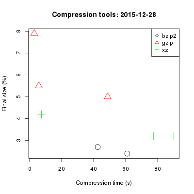
There are three major file compression tools on linux, the venerable gzip, bzip2, and the newer xz. I tried them out on a 285MB NetCDF file, one of the very many I’m working with. I included most compression (-9) and fastest (-1) options for each of the three tools, plus the default (-6) for gzip and xz. bzip2 doesn’t have the same range of options, just best (the default) and fast.

There wasn’t a huge difference in compression for this type of file, with the best (bzip2 -best) resulting in 2.4% of the original, and the worst (gzip -1) in 7.9% of the original size.

Speed, though: anywhere from 2.9 to 90.0 seconds to compress a single file. Uncompression time was about 1.6 seconds for gzip and xz regardless of option, and 3.2-3.6 for bzip2.

Compression tool results

For this file format, xz was useless: slow and not the most effective. bzip2 produced the smallest files, but not by a huge amount. gzip was fastest, but produced the largest files even on the best mode.

This matches what I expected, but the specifics are useful:

  • Using bzip2 -best I could get one set of files from 167GB to 4GB, but it would take 9.5 hours to do so.
  • Using gzip -1 I could get that set of files down to 13GB, and it would only take 24 minutes.

I think that’s a fair trade-off. The extra 9 hours is more important to me than the extra 9GB, and accessing a single file in 1.5 seconds instead of 3.5 also improves usability on the occasions when we need to access the raw data.